Choosing Between SigLIP and CLIP for Language Image Pretraining
| Ritwik Raha | Aritra Roy Gosthipaty |
| Machine Learning Engineer | Machine Learning Engineer |
| ritwik_raha | arig23498 |
Introduction
Suppose are given an image and three different captions. One of the captions correctly describes the image. How would you, as a human, choose the correct caption?
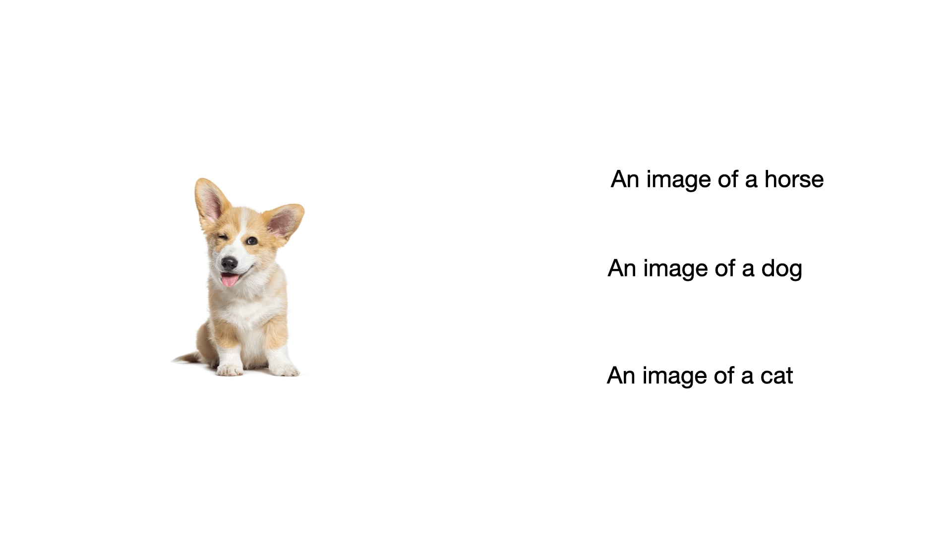
You first look at the image and understand what is in it.
See the captions and grasp what is written.
Compare the representation of the image with the captions.
The caption which corresponds most to the image is your choice.
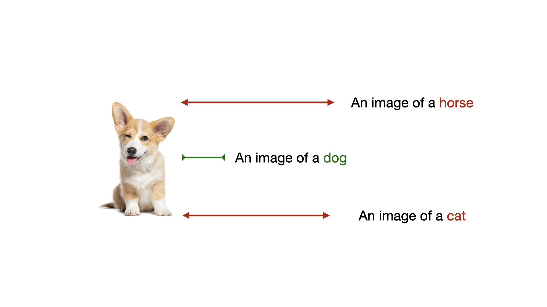
How can we use a deep learning model to achieve this
To make our deep learning model choose from the caption, we need two models one for the image and one for the text. The image model takes the image as an input and outputs the visual representation in terms of image embeddings. The text model takes the captions as input and outputs the textual representation in terms of text embeddings.
We know that embeddings are vectors in a higher dimensional space. To compute the similarity between vectors, we compute the cosine similarity between them. Similarly to compute the similarity between the text and image embeddings, we compute the cosine similarity between them.
This task (choosing the correct text and image pairs) is a great pre-training objective for vision and language models. To simplify, the image and text embeddings for the correct pair should be similar, while that of the incorrect pair should be dissimilar.
We can formulate the task in a couple of ways. In this blog post, we talk about two prominent ways introduced in CLIP and SigLIP, and understand which is better (here there is a clear winner).
How does CLIP do it?
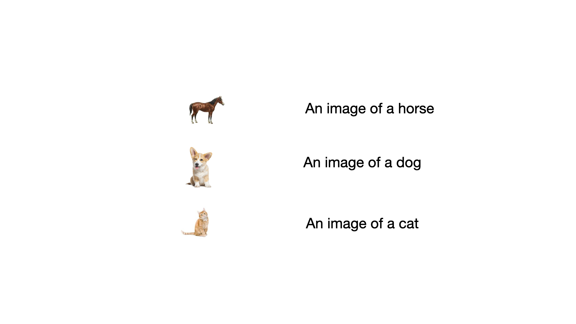
The figure below is what a mini-batch of data for our task (choose the correct pair) looks like. A collection of image-text pairs. We denote images with I and text with T.
$$\text{Mini Batch } \mathcal{B} = \{(I_1, T_1), (I_2, T_2) \dots\}$$
CLIP (Connecting Text and Images by OpenAI) devises two models, an image encoder and a text encoder.
$$\text{Image Encoder: } f(I)=x$$
$$\text{Text Encoder: }g(T)=y$$
The encoder, as the name suggests, takes the input and encodes it into a latent representation (denoted by x for image latent, and y for text latent).
Now that we have the embeddings (the latent representations) from the encoders, we need a way to compute the similarity score. We delegate this to our friendly neighborhood function "the dot product".
$$\text{Dot product: }x.y$$
The similarity score gives us a measure of how similar the image and the text embeddings are. We would need to figure out a way to transform the similarity score into a likelihood measure.
Why a likelihood measure? We want to predict (deep learning models are tasked to predict) how likely a text and an image pair are.
To get the likelihood measure we use the soft-max function.
$$\frac{e^{\text{similarity score of a correct pair}}}{\sum_{\text{all incorrect pairs}}e^{\text{similarity score of pairs}}}$$
The numerator only deals with the correct pairs, while the denominator deals with everything except the correct pair. Intuitively the denominator is the normalization term, which makes the equation transform a similarity score into a likelihood measure.
Now that we have our likelihood measure, we can apply a log to it and then turn the product of likelihood into a summation (a trick deep learning engineers use quite often).
To condense this section into a mathematical statement we can write:
$$\sum_{i=1}^{|\mathcal{B}|}\left(\log\frac{e^{x_{i}y_{i}}}{\sum_{j=1}^{|\mathcal{B}|}e_{x_{i}.\boxed{y_{j}}}}\right)$$
If you look closely you will know that the image is static while we loop over the text in the mini-batch (the boxed section).
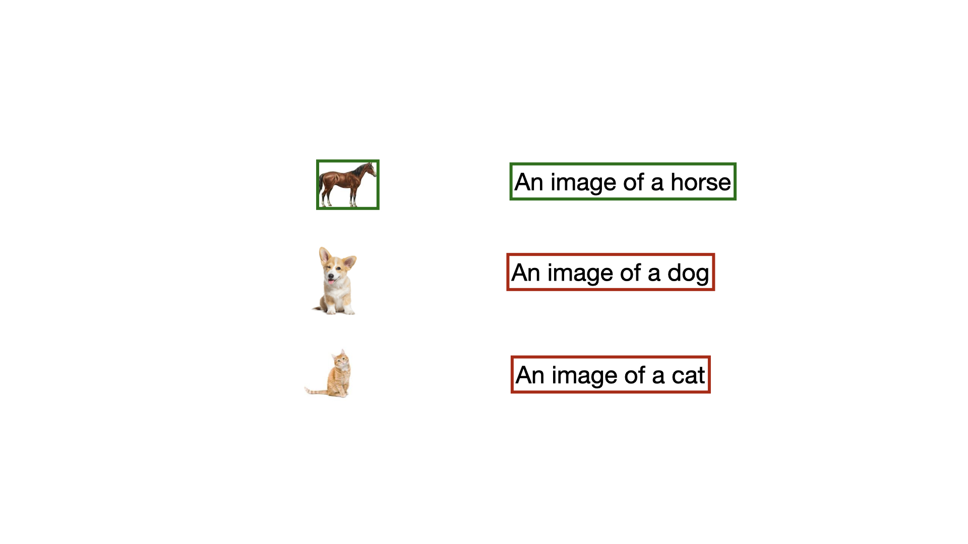
In CLIP we also keep the text static and loop over the image, to build the complete loss function.
$$\sum_{i=1}^{|\mathcal{B}|}\left(\log\frac{e^{x_{i}y_{i}}}{\sum_{j=1}^{|\mathcal{B}|}e_{\boxed{x_{j}}.y_{i}}}\right)$$
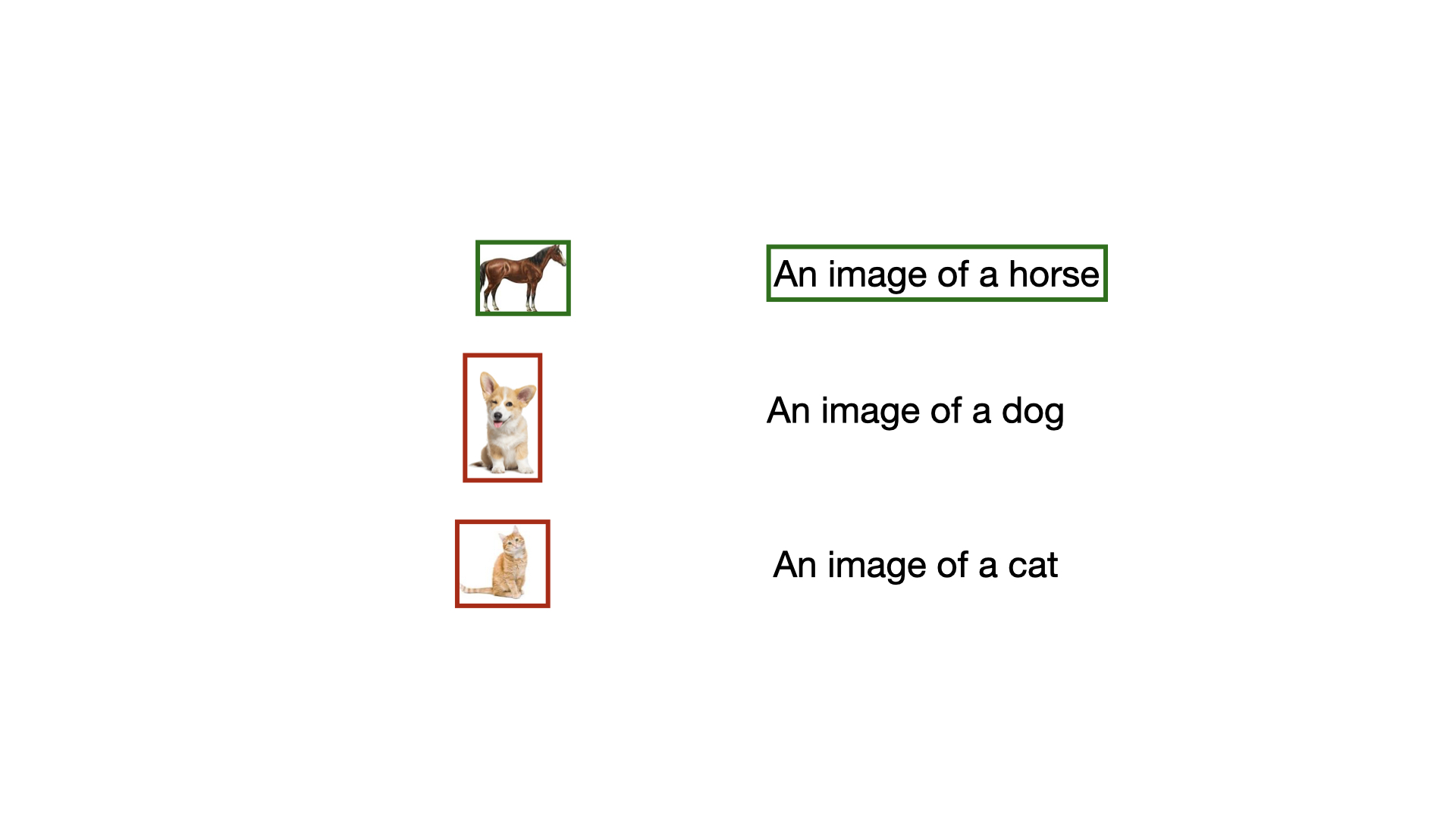
Is soft-max bad?
We now know that the loss function used in CLIP from OpenAI is similar to a soft-max function. We needed soft-max to convert our similarity scores into likelihood estimates. The main reason for this transformation is the normalization term (the denominator).
Let's now take a different mini-batch of our dataset as shown in the Figure below. If you were to think of a problem with this mini-batch, what would that be?
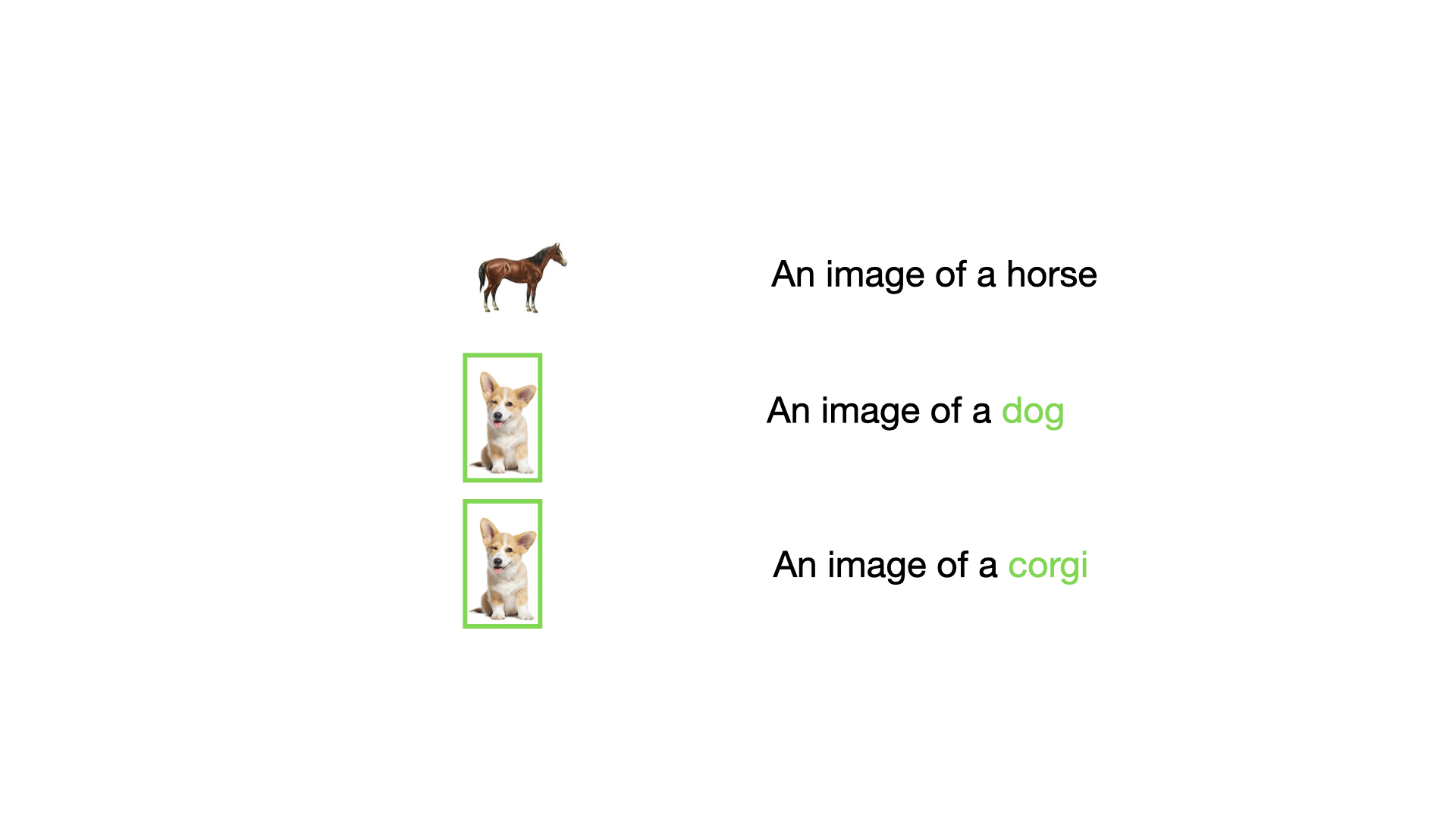
The data at index 2 and 3 (dog and corgi) are very similar to each other. This will harm the normalization term in the soft-max, which in turn harms our mini-batch loss. Here we uncover a very important assumption that needs to be in place to use the CLIP loss:
The mini batch should not have similar data points.
Problem 1: This is genuinely a very difficult problem to solve. We have to get into our dataset, apply a filter (semantic filter of sorts), and prune the dataset before training our model.
Problem 2: Let us now focus on a different problem. The soft-max loss is batch dependent. Even if you prune the dataset very well, you would need a big (in orders of thousands) batch size to train the model. The batch size problem directly stems from the normalization term. The more varied data present in a mini-batch, the better likelihood term we get!
Problem 3: Notice that the loss function of CLIP runs twice in the training loop. Once where the image is static we iterate over the text, and the other time when we keep the text static and iterate over the images.
The three major cons:
Pruning dataset is a must
Large batch size is a must
Running the loss function twice is a must
All of these problems motivated researchers to devise a better (more data and batch-agnostic way) to compute the loss.
Enter SigLIP
If you think about the root cause of all the cons of soft-max loss, you will quickly notice that it is the normalization term (the denominator).
The denominator is a sum of the exponential similarity score of all the other pairs except the correct one.
How do we get rid of the normalization term?
SigLIP (Sigmoid Loss for Language Image Pre-Training) a 2023 paper from Google DeepMind aims to solve this problem with the sigmoid loss expression.
The Sigmoid Loss
Let's first check out how the sigmoid function looks like:
$$y=\frac{1}{1+e^{-x}}$$
Note, here x and y are the coordinates of a 2D plane. If we plot the graph we get something like this:
What if we just used sigmoid instead of softmax?
That is exactly what the authors of SigLIP did, formulate the language-image pretraining objective as a sigmoid loss function.
The sigmoid loss used in SigLIP can be represented as follows:
$$L = -\frac{1}{|B|} \sum_{i=1}^{|B|} \sum_{j=1}^{|B|} \log \frac{1}{1 + e^{z_{ij}(-tx_i \cdot y_j + b)}}$$
Instead of the softmax, SigLIP uses a sigmoid-based loss that operates independently on each image-text pair. The pseudocode from the Google Deepmind paper is presented below:
# img_emb
# txt_emb : image model embedding [n, dim] : text model embedding [n, dim]
# t_prime, b : learnable temperature and bias
# n : mini-batch size

t = exp(t_prime)
zimg = l2_normalize(img_emb)
ztxt = l2_normalize(txt_emb)
logits = dot(zimg, ztxt.T) * t + b
labels = 2 * eye(n)- ones(n) #-1 with diagonal 1
l =-sum(log_sigmoid(labels * logits)) / n
Let us understand the design of this loss function in detail:
-1/|B|: Scales the loss by the inverse of the batch size, ensuring the loss is comparable across different batch sizes.Σ(i=1 to |B|) Σ(j=1 to |B|): Computes the loss over all possible image-text pairs in the batch, including both positive and negative pairs.log(·): Converts the probability from the sigmoid function into a loss value. It helps in numerical stability and makes the optimization landscape smoother.1 / (1 + e^(·)): Maps the input to a probability between 0 and 1. For positive pairs, we want this probability to be high (close to 1), and for negative pairs, we want it to be low (close to 0).z_ij: Determines whether the pair is positive (1) or negative (-1). It flips the sign of the similarity for negative pairs.t: Controls the steepness of the sigmoid. Higher values make the model more confident but potentially less stable. Lower values make it less confident but more stable.x_i · y_j: Measures how similar the image and text embeddings are. Higher values indicate more similar pairs.b: Shifts the decision boundary of the sigmoid. It helps to counteract the imbalance between positive and negative pairs, especially at the start of training.
def sigmoid_loss(image_emb, text_emb, temperature, bias):
    similarity = dot_product(image_emb, text_emb)
    logits = temperature * similarity + bias
    labels = 2 * eye(batch_size) - 1  # 1 for positives, -1 for negatives
    loss = -mean(log_sigmoid(labels * logits))
    return loss
Architecture of SigLIP
Here's a high-level view of how data flows through the SigLIP model:

The authors of the Google DeepMind paper pre-trained their SigLIP models on the WebLI dataset, using only English image and text pairs.
The authors used moderately-sized models: B/16 ViT for image embeddings and B-sized transformer for text embeddings.
The input images were resized to 224×224 resolution.
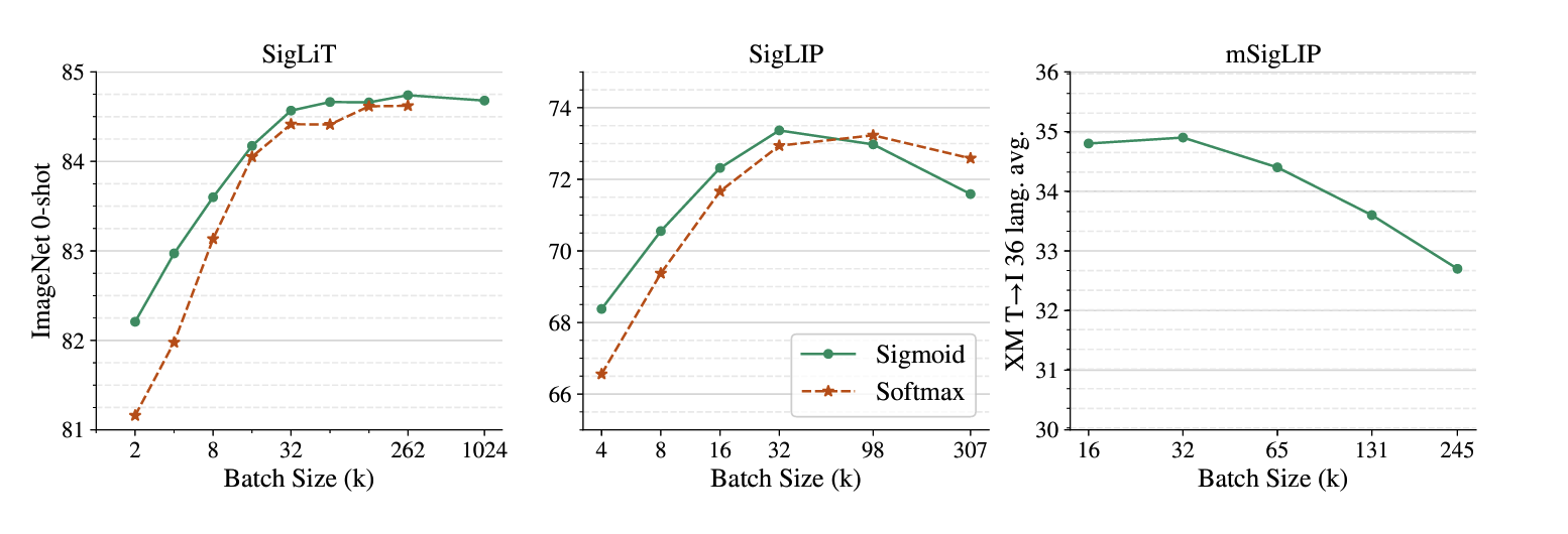
The text was tokenized by a 32k vocabulary sentence-piece tokenizer trained on the English C4 dataset, and a maximum of 16 text tokens were kept. Figure 2 middle plot shows SigLIP results.
With less than 32k batch size, SigLIP outperformed CLIP (WebLI) baselines.
On the other end of the scale, the memory efficiency of the sigmoid loss enabled much larger batch sizes.
For example, with four TPU-v4 chips, they could fit a batch size of 4096 with a Base SigLIP but only 2048 with a corresponding CLIP model.
Analysis of Batch Size Effects
One of the most intriguing aspects of the research was a comprehensive study on the impact of batch size in contrastive learning. This study challenges some common assumptions and provides valuable insights for practitioners.
The authors followed the setup from the Locked-image Tuning (LiT) paper. The DeepMind authors explored an unprecedented range of batch sizes, from 512 to 1 million, to thoroughly investigate the relationship between batch size and model performance.
Observations
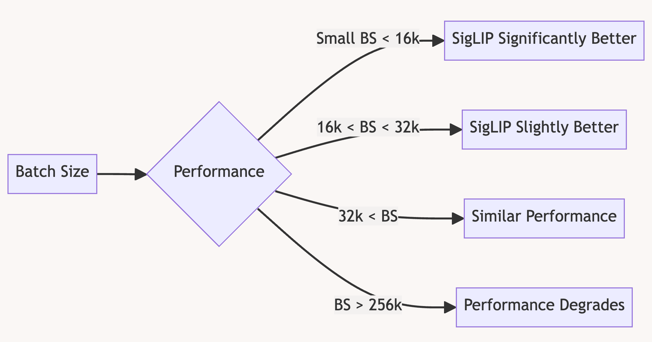
SigLIP performs well with smaller batch sizes, both losses stabilize around 32k, and very large batch sizes (>256k) can reduce performance.
Sigmoid vs Softmax Performance
For batch sizes < 16k: Sigmoid loss significantly outperforms softmax
For batch sizes > 16k: Softmax catches up, with sigmoid slightly ahead
Performance Saturation
Surprisingly, performance saturates around 32k batch size
Further increases yield only minor improvements
Peak performance observed at 256k batch size
Large Batch Training
Successfully trained a SigLiT model with a 1 million batch size
This is far beyond previous studies, which typically stopped at 64k
Best Performance
The authors mention their best SigLiT model (B-sized text encoder) achieved 84.7% zero-shot ImageNet accuracy
The original LiT paper reported 85.2% with a 10x larger text model
The batch size study reveals that the relationship between batch size and performance in contrastive learning is more nuanced than previously thought. While larger batch sizes can yield better results, there's a point of diminishing returns (around 32k in our experiments).
The sigmoid loss consistently performs well across batch sizes and enables efficient training with limited resources. This makes SigLIP a versatile choice for various research and production scenarios.
Future Directions and Open Questions
How can we further improve efficiency for multilingual training?
Are there ways to combine the benefits of sigmoid and softmax losses?
Can we design more effective negative sampling strategies for the sigmoid loss?
How does SigLIP perform on other modalities beyond images and text?
Conclusion
So clearly SigLIP is better and we must strive to "find-and-replace" CLIP with SigLIP across all code bases and all researches right?
We must replace CLIP with SigLIP right?
Well, the answer is not so simple. As illustrated above batch size, compute resources and pretraining strategy play a massive role in the choice of the loss function.
Contrastive Losses in Vision Language Models
Contrastive loss functions are crucial in training vision-language models because they help the model learn to distinguish between correct and incorrect image-text pairs. By maximizing the similarity of correct pairs and minimizing the similarity of incorrect pairs, the model can better understand and match images and text.
Use CLIP: When you have access to large computational resources and can handle the need for large batch sizes and dataset pruning.
Use SigLIP: When you want a more efficient training process, especially with limited computational resources. SigLIP is also preferable when you need to train with smaller batch sizes.
Use Custom Loss: When you have specific requirements or constraints that neither CLIP nor SigLIP can address, designing a custom loss function tailored to your needs might be the best approach.
SigLIP demonstrates that sometimes, simpler is better. We can achieve impressive results with improved efficiency by rethinking the fundamental loss function for contrastive learning. This work opens up new possibilities for scaling language-image pre-training and making it more accessible to researchers with limited computational resources.


